Toolchain Pipeline

Toolchain Pipeline

Processing Order

Everything that happens to an image, from the moment you open the file to the moment it is displayed on screen or saved, takes place in a fixed order. The data flows from one module to another - this is the toolchain pipeline. RawTherapee contains four pipelines (one for the main preview, one for the saved image, one for the thumbnail, and one other that currently escaped me). The following list shows a simplified order of operations:

1. Preprocess
   1. Dark frame
   2. Flat field
   3. Bad pixels
   4. Hot pixels
   5. Scale colors (internal, no tool in UI)
   6. Raw black point
   7. Lens distortion correction
   8. Green equilibration
   9. Line noise filter
   10. Chromatic aberration Correction
   11. Raw white point
   12. Raw histogram
   13. Prepare Auto Exposure
2. Demosaic
3. Retinex
4. Highlight recovery
5. White balance
6. Spot Removal
7. Crop
8. Convert colorspace
9. Noise reduction
10. Dehaze
11. Dynamic range compression
12. (Local Adjustments branch) avoid color shift, Log encoding, blur-noise denoise, tone-mapping, dehaze & retinex, contrast by detail levels, vibrance, soflight, local contrast, wavelet, sharp, exposure, color and light, Color appearance (Cam16 & JzCzhz), avoid color shift
13. Auto-match tone curve
14. Tone response curve
15. Process RGB
    1. Channel mixer
    2. Tone curve
    3. Highlights
    4. Shadows
    5. RGB curves
    6. HSV curves
    7. Color toning
    8. Film simulation
    9. Black-and-white
    10. L*a*b* color correction grid (Lab)
16. Process Lab
    1. Shadows/Highlight (Lab)
    2. Local contrast (Lab)
    3. Lab adjustements
    4. Vibrance
    5. L*a*b* color correction grid (Lab)
    6. Vignette filter
    7. Graduated filter
    8. Tone mapping
    9. Impulse noise reduction
    10. Defringe
    11. Edges
    12. Microcontrast
    13. Sharpening
    14. Contrast by Detail Levels
    15. Wavelets
    16. Soft light
    17. Abstract Profile
    18. CIECAM02
    19. Resize
    20. Post-resize sharpening
17. Final Lab -> RGB conversion

List of All Tools in RawTherapee

• Generic/Main preview
  • Input profile
  • Monitor Color Profile
  • Working profile
  • Output profile
  • Clipping indication
  • Red/Green/Blue/Luminosity/Focus mask previews
  • Colorimetric intent
• Exposure Tab
  • Exposure
  • Shadows/Highlights
  • Tone Mapping
  • Dynamic Range Compression
  • Vignette Filter
  • Graduated Filter
  • Lab Adjustments
• Detail Tab
  • Sharpening
  • Local Contrast
  • Edges
  • Microcontrast
  • Impulse Noise Reduction
  • Noise Reduction
  • Defringe
  • Contrast by Detail Levels
  • Haze Removal
• Color Tab
  • White Balance
  • Vibrance
  • Channel Mixer
  • Black-and-White
  • HSV Equalizer
  • Film Simulation
  • Soft Light
  • RGB Curves
  • Color Toning
  • Color Management
• Advanced Tab
  • Retinex
  • CIE Color Appearance Model 2002
  • Wavelet Levels
• Transform Tab
  • Crop
  • Resize
  • Lens/Geometry
    • Rotate
    • Perspective
    • Profiled Lens Correction
    • Distortion Correction
    • Chromatic Aberration Correction
    • Vignetting Correction
• Raw Tab
  • Sensor with Bayer matrix
    • Demosaicing
    • Raw Black Points
    • Preprocessing
    • Chromatic Aberration Correction
  • Sensor with X-Trans matrix
    • Demosaicing
    • Raw Black Points
  • Raw White Points
  • Preprocessing
  • Dark Frame
  • Flat-Field
  • Film Negative
  • Capture Sharpening

RawTherapee pipeline : linear or non-linear ?

Linear processing: what is it and why is it used?

In the so-called scene-referred workflow images are processed using linear operations. This occurs up until the point where the scene values are converted to display-adapted values (output tone mapping). The L*a*b* colour space is avoided in the intermediate steps prior to the output transform. The claimed advantages are as follows:

• Working in linear RGB is simpler, the algorithms are faster and can tolerate more extreme adjustments without generating artifacts.
• Avoids the use of the L*a*b* color space which supposedly limits the dynamic range and introduces hue and saturation shifts.

RawTherapee takes a different approach while still meeting the desired criteria in terms of dynamic range, hue integrity and minimum artifacts.

Linear maths

Linear operations include polynomials, linear equations, vector transformations, matrix calculations, the Fourier transform, Wavelets, etc. They do not include logarithmic or exponential functions, exposure, gamut compression, hyperbolic functions, tone curves, L*a*b* or CIECAM, etc.

What happens when you take a photo?

The camera’s sensor, whose internal characteristics are largely unknown, is exposed to a natural or artificial illuminant or multiple illuminants, falling on a subject for which precise color information is unknown (i.e. spectral data for each part of the image - flowers, animals, buildings, etc.). Not only that, but the tristimulus “observer” values produced by the camera are different to those of a human observer.

Each illuminant is either:

• natural light, governed by the time of day, the amount of cloud cover and the laws of Planck and Boltzmann (a combination of quantum and wave physics);
• artificial, with a spectral distribution that is usually unknown.

What we can say for certain is that the data recorded on the sensor and perceived by our eyes cannot be defined using linear algebra. This observation raises the question: should we strive to process data linearly when, by its very nature it is not, or that this data is subject to uncertainty, especially when there are LED illuminants? Consider our digital cameras, they attempt to use a 3x3 (linear) matrix and a D65 illuminant (6500K), an admission of our inability to do better.

What is important?

We need to distinguish between the part of image processing that aims to best “map” the data recorded on the sensor into the working profile, which is done in true 32- or 64-bit (lossless) mode and the visualization part, whether on a screen or to a printer. For the latter, the gamut is often much narrower and a curve simulating our visual perception (gamma) is also applied. Currently, the majority of display conversions are done in 8-bit L*a*b*, which results in a considerable loss of data. Obviously any further processing after such a conversion should be avoided.

Factors affecting data linearity

In addition to illuminants as mentioned above, the following non-exhaustive factors can be cited:

• The recovery of highlights and shadows for example. Color Propagation attempts to restore values up to 4 to 10 times the usual maximums (beyond the working profile). It seems obvious that it is highly desirable to bring this data back into the human-visible range i.e. the working profile, otherwise we’re just making things up by manipulating imaginary data. Subsequent processing on the working-profile data should remain unbounded.
• Gamut compression, which aims to make out-of-gamut data (whether related to the illuminant or to exposure) consistent with the output gamut.
• White balance, which ultimately boils down to three multiplication coefficients, but which in reality involves complex phenomena that are difficult to model e.g. in Temperature Correlation.

The choices made in RawTherapee

Faced with these difficult challenges given that there are many more unknowns than equations, RawTherapee proceeds as follows :

• Treat what can be treated using linear algebra even though we often lack all the necessary information and are obliged to use simplified models. We also need to bear in mind that processing image data that falls outside the limits of the working profile is a daunting task and a risky gamble because we are dealing with imaginary colors and cannot visualise what we are doing. These operations can be referred to as sensor-referred processing.

• Use linear, logarithmic, or hyperbolic transformations to fit the data (without limiting) into the working profile to :

  • bring the black point close to zero to optimize contrast,
  • adjust the highlights asymptotically and reduce the dynamic range,
  • prepare it for the visualization stage by reducing the gamut (often in 8 bits) and applying a gamma adjustment.

• With the exception of the final display conversion to 8 bits, these transformations are performed in unbounded 32-bit (or 64-bit) floating-point format, without data loss, and are often reversible. For example, the RGB -> L*a*b* and L*a*b* -> RGB transformations, which also preserve the colorimetry using a Munsell correction, are capable of handling a dynamic range of at least 25 Ev.

• Multiple algorithms can be used (for example, General Hyperbolic Stretch combined with Abstract Profile) to optimize the data.

• Use CIECAM either at the end of the processing pipeline just before the output-device conversion (monitors, printers, etc.), or in conjunction with Selective Editing, to best account for physiological effects that are misinterpreted by mathematical algorithms alone. In particular, this includes the physiological effects of the shooting or scene conditions (simultaneous contrast, Hunts effect, etc.) and the viewing conditions.

Finally RawTherapee sets out to ensure that throughout the process:

• the data prior to the final conversion remains within the working profile by using the histogram in linear mode and ensuring that you avoid using or generating imaginary colors (for example, manipulating primary colors is risky);
• the entire process leading up to the final conversion stays within the gamut limits of the output profile.

Conclusion

There is no single correct approach to processing raw files. What is important is that the process of preparing the data for display does not introduce unnecessary data loss or limitations that can compromise the end result.

RawTherapee takes a different approach from other software; in RawTherapee the concepts of “scene-referred” and “display-referred” are not strictly used (except with some similarities when using processes based on CIECAM). This doesn’t mean that the scene-referred concept isn’t effective when used in the appropriate context.

L*a*b* is used when appropriate because in 32-bit mode, it allows for a dynamic range of at least 25 EV and avoids color shifts (to maintain nearly perfect hue linearity) by using Munsell correction.

The approach to processing in RawTherapee is based on the following general combination:

• Optimize the RAW data using linear algebra (demosaicing, black point adjustment, capture sharpening, etc.);
• Use gamut compression to manage the output profile gamut from the very beginning of the process;
• Use a white-balance method based on temperature correlation when possible, rather than conventional white balance;
• Use the concept of “pre-tone mapping” to bring the current black point close to zero, manage highlights asymptotically, and reduce the “dynamic range” to bring the data back into the working profile and obtain an “acceptable” image for further processing.
• Adjust tonal contrast, highlights, and tone mapping to prepare the output, without limiting the data.
• Adjust colors while taking into account the physiological aspects of colorimetry along with the shooting and viewing conditions, without limiting the data, for example CIECAM.

This approach does not conflict with the principles of scene-referred or display-referred processing, but interprets them differently from what is done elsewhere, allowing for greater flexibility. The goal is the same. The principles outlined above should be viewed as a guide rather than a rigid framework. Each image is a unique case and the processing needs to be adapted accordingly. You can get a glimpse of this approach in the two Rawpedia tutorials:

Game Changer

RawTherapee Process Challenge

Colorimetry

The Importance of CIECAM and L*a*b*

Colorimetry gives rise to a lot of debate but we have to remember that it is not an exact science. No amount of equations, however complex, can ensure that the human eye will necessarily be satisfied with an image.

Currently RawTherapee uses the L*a*b* color space and CIECAM02/16 for chromatic adaptation and work has begun on exploring other color spaces (Jzazbz) and CAM models, for HDR applications (ZCAM does not work)..

The use of the L*a*b* (or CIELAB) color space does have its limitations but many of its shortcomings can be successfully mitigated, at least for SDR applications.

For example:

• One of the most frequent criticisms is that L*a*b* is non-linear and that it “distorts” the colors, in particular for blue-violet and red-orange. This is certainly true if you simply adjust the image using curves or chromaticity sliders. However in RawTherapee, if you click on “Avoid color shift” (Munsell correction), nearly 200 LUTs will correct these shifts and make the image perfectly linear.
• It is also said that L*a*b* addresses imaginary colors if the working profile allows it. This is also true but again, this can be compensated in RawTherapee by enabling “Avoid color shift”. In this case, a relative colorimetric correction is applied to the working gamut as follows:
  • It analyzes the image data.
  • If it is within gamut no action is taken.
  • If it is outside gamut,the chroma is reduced and if this is insufficient, or if it is close to L=0 or L=100, then L is adjusted.
  • You can also choose the algorithm developed by Emil Martinec (gamutmap) which provides XYZ control (absolute or relative).
  • However this should rarely occur if Prophoto is used in the Working Profile and is probably not important.
  • If the saturation has been adjusted (chroma, vibrance,…), a Munsell correction using nearly 200 LUTs is applied. This will correct any color shifts with a high degree of accuracy e.g a red that has turned orange because of L*a*b*, will become red again. There will still be some errors but they are very small.
  • The Munsell correction is applied in all cases unless none is selected.

L*a*b*

• L*a*b* is a reversible transformation of XYZ (in simplified terms, Y is transformed into L* using a gamma of 3.0 and a slope of 9.03). L*a*b* has more or less the same characteristics in terms of its limits (those of the primaries) as XYZ, which serves as a reference for the Working Profile and determines the basis of the gamut. Therefore L*a*b* and XYZ have essentially the same characteristics (exposure range, gamut, etc.). One point however, in many processes the values of L* can be bounded (clipped), to limit artifacts (high contrasts, highlights…), but in most cases L* is unbounded. If we ever get to HDR processing, we’ll probably have to switch to “HDR-Lab”. The data is not lost, even for high-dynamic range images (>= 25Ev), but the progression in the highlights is not progressive enough when used with monitors capable of displaying luminance values in the range of 120 cd/m² and beyond.
• I don’t think that the RGB->Lab transformation itself prevents complete HDR processing. This is because the calculations are generally carried out using ‘float’ or ‘double’ data values (32 or 64 bits) or using SSE (128 bit - 4x32 or 2x64 bits). The linear part of the Lab transform allows shadows with values of 0.005 cd/m2 or less to be processed. The parabolic part (gamma = 3.0) limits the distribution of data in the highlights allowing them to be reproduced more accurately (on suitable monitors) with luminance values above 120 cd/m2. The XYZ<=>Lab conversion leads to hardly any loss of data (insignificant due to double conversions) and can be considered as a kind of lossless compression. Of course if we want to achieve complete HDR processing, it is necessary to ensure that the way the data is processed, prior to being sent to the monitor, allows for more progression in the highlights. The preferred approach for Rawtherapee would be to implement HDR-Lab instead of Lab. But in the meantime I have implemented the possibility of changing the gamma of Lab (3.0) for several tools (wavelets, tone-mapping, etc.) notably to make it linear. It should be noted that Rawtherapee is designed to overcome one of the problems with Lab, which is the non-preservation of the hue when the saturation changes (especially in oranges and purples), by using “Perceptual Uniform Lab”. This involves using a series of Munsell LUTs, as well as gamut control to prevent virtual colors.

L*a*b* does not impact the gamut or the dynamic range of high-dynamic-range images as shown in the following example with a Dynamic Range of 25Ev

Note that the majority of digital cameras in 2024 have a maximum dynamic range of about 15Ev. This image is therefore exceptional but demonstrates the behavior of Lab* for images with a high dynamic range.

TIF file (Creative Common Attribution-share Alike 4.0): 1

Original image - 25Ev - unprocessed

Note:

• The shadows lack detail.
• Approximately 40% of the image is 100% white.
• The restored black-to-white dynamic range is around 12 to 13 Ev.

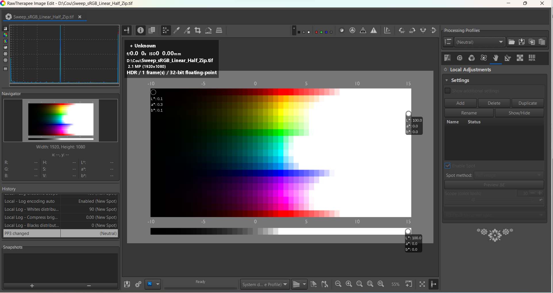
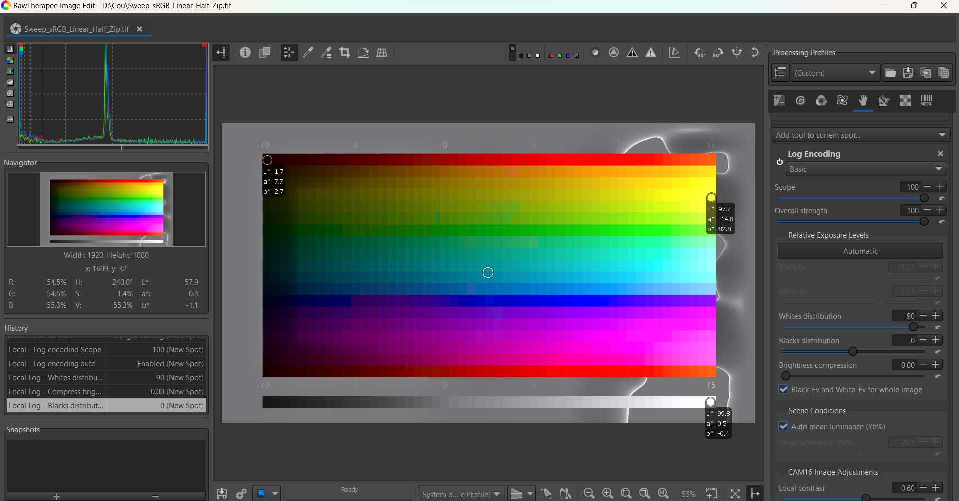
Image with Local Adjustments - Log Encoding

Note:

• The shadows and highlights occupy the entire visible range from L=1 to L=99.8 (scale 0 – 100).
• The colors appear evenly distributed as a function of luminance. The use of L*a*b* does not impact the dynamic range.
• The dynamic range of the blacks, whites and color is restored to 25Ev.
• Note the use of “White distribution = 90”.

CIECAM02/16

• One criticism of Ciecam02 is that is not able to process high dynamic range and wide color gamut images, which is partially true. A number of improvements were made by the development team a few years ago to mitigate this problem (bearing in mind that a large number of user images fall within the sRGB gamut and do not pose a problem). However, by using Log Encoding in conjunction with Cam16, or Color appearance (Cam16 & JzCzHz), the vast majority of problems can be solved. Of course some images will still present problems, in particular with highlight reconstruction, but this is not specific to Ciecam. The addition of Ciecam16 (Cam16) solves some of these problems.
• Ciecam02/16 is one of the only ways to achieve true colorimetric correction because it takes into account human perception and the surrounding environment. With Ciecam for example, any adjustments to the luminosity and/or the saturation, will take into account the image and its environment.

White Balance

• White balance is also subject to debate. The Temperature Correlation module recently introduced in Rawtherapee is almost mathematically (cognitively) perfect. It makes the xyY colors of the image coincide with known spectral data. However, on images where the temperature deviates a long way from D50, the colorimetry will not be correct because there will not be the necessary chromatic adaptation expected by our eyes and brain. Ciecam however, can take this into account.

Importance of the Linear-RGB Model and Colorimetry

The merits of the RGB model, and in particular, the linear RGB model are frequently cited. It is certainly the best way to carry out “upstream” processing (demosaicing, white balance, defringing, chromatic aberration correction, etc.) and anything that can be done in this mode should be.

However, CIELAB and Ciecam02/16 still have their place despite their shortcomings. As we have seen above, they are both derived from the CIE XYZ tristimulus values with Ciecam being one of the only ways to achieve true colorimetric correction.

So what about tone curves?

• Not only are they non-linear but they only provide limited colorimetric compensation, if any (with the exception of the Perceptual mode, which uses Ciecam02). This is in contrast to the Tone Response Curves -TRC- used for output (monitor, TIF etc.).
• The Auto-Matched Tone Curve, which is a copy of the in-camera TRC, is applied mid-process and introduces non-linearities in the processing pipeline.

What about saturation?

• Maintaining RGB linearity when you change the saturation is not impossible but it is difficult and is not implemented in Rawtherapee. On the other hand, if you adjust the saturation using Ciecam, it will take into account variations in luminance (or brightness) and adapt the color accordingly.

In conclusion, RGB, L *a *b *, and Ciecam all have their advantages and disadvantages. They simply need to be understood so that they can be used appropriately.

What are the acceptable principles for processing SDR or HDR images?

The argument below is partly based on the fact that Rawtherapee has two Ciecam modules, one located at the end of the main process (Color Appearance & Lighting), the other in Selective Editing, Color Appearance (Cam16) located just after white balance. These 2 modules are Color Appearance Models (CAMs) and contain all the processes and tools needed to ensure good colorimetry. However, these 2 modules alone are not always able to process: a) images with a very high dynamic range, b) images with very pronounced shadows, c) images with strong highlights (not to be confused with highlight reconstruction).

The science of colour matching is often inexact and imprecise. Nevertheless, as we have seen, the most linear treatment possible seems to be recommended if practicable. However, this seems impossible if the differences linked to a) b) c) above are significant. In these cases, I propose as a first step a principle close to that of the rendering of human vision: a linear part (slope) to ‘unblock’ the shadows and a parabolic part (gamma) to render the perception of medium tones and highlights fairly similar to that of our eye/brain pair. This linear/parabolic differentiation is commonly used in various software applications e.g., sRGB gamma where Slope =12.92 and Gamma=2.4, or BT709 where slope=4.5 and Gamma=2.22 or ‘Lab’ where Slope=9.03 and Gamma=3.0. The two Tone Response Curve (TRC) modules present in the Abstract Profile module or in Selective Editing > Color Appearance > Source Data Adjustments provide a partial response to the problems described in a) and b), by allowing adjustments to be carried out with higher Slope and Gamma values.

The problem of reducing highlights, improving overall contrast and using local contrast still remains and will be discussed below.

Don’t forget that Cam16 is a processing module in its own right. You can use it to process images using tools such as:

• Surround or Scene conditions ( average, dim, dark etc.) which allows you to take dark or very dark backgrounds into account. This algorithm alone can provide shadow enhancement in certain images.
• Lightness, Brightness (and their corresponding contrast parameters), Chroma, Saturation, Colorfulness, etc.

Selective Editing - Cam16 and HDR functions

As mentioned above, colorimetry is not an exact science so you should use whichever tools give a result that is pleasing to your eye.

How useful are ICC and DCP input profiles ?

Raw files are generally decoded using a matrix (from Adobe) called ‘Color Matrix1’ based on the D65 illuminant. This matrix is sufficient in the vast majority of cases. It can be replaced by either an ICC profile or a DCP profile that has been developed either by the user, using a Colorchecker24 for example, or supplied by Rawtherapee or Adobe. There are two broad problems with these sorts of profiles:

• The Colorchecker24 is limited (with one exception in blues) to the sRGB gamut. What happens when such a profile is used, for example, on images of flowers or minerals where the gamut is much larger?
• The profile is only really relevant for a given illuminant. What happens when a profile developed for D50 (daylight in the sun) is used in the shade? It is true that DCP profiles have an interpolation table between D65 and Tungsten 2850K, but this is still approximate.

My point is not to say that you shouldn’t use these profiles, which are very useful for reproducing paintings, coins, etc. in controlled lighting, but to show their limitations.

Should I use the Auto-Matched Tone Curve?

The answer is: maybe? This curve generated from the JPEG attached to the Raw reproduces the colourimetry of the camera manufacturer (Canon, Nikon, Sony, etc.). This is a criterion of choice, but it has a few constraints:

• The generated curve can lead to an increase in contrast which, depending on the image, may cause clipping in the shadows and highlights. In many cases, this increase in contrast is undesirable.
• The default choice of ‘Film-like’ modifies the colorimetry. This modification contradicts the underlying philosophy of Ciecam. If you want to keep the Auto-Matched Tone Curve, it is better to use the Standard mode.

Should I use the Exposure module, and in particular ‘Exposure compensation’?

The answer is: with reservations. In the case of images of type a), b) or c), the Exposure slider will bring about a linear change in exposure (in Ev), increasing (or reducing) shadows and highlights in the same way. The ‘Highlight compression’ and Blacks sliders can be used to mitigate this but the adjustment is not very intuitive and can conflict with the TRC Gamma/Slope adjustments. An alternative is to use the Tone Equalizer (in the main menu or in Selective Editing), which allows progressive differentiation of highlights and shadows.

Tone-mapping modules - description and use

I’ll only focus on the modules using Black Ev, White Ev and ‘Mean Luminance (Yb%) Scene’. For the other Rawtherapee tone mapping modules are concerned:

• Tone Mapping is more a module for significantly modifying the local contrast (texture) than for carrying out a true tone mapping.
• Dynamic Range Compression uses a Laplacian and a Fourier transform. Its performance is OK, but it is slow and consumes a lot of resources.
• Note that most images - even with modern cameras - are limited to 14 or 15 Ev. HDR software that produces a DNG image from several bracketed images should be able to reach around 20 Ev.

An evaluation of the dynamic-range capabilities of tools in Selective_Editing 2

The principle of calculating Dynamic Range (DR)

Three algorithms use the concepts associated with Dynamic Range i.e. Black Ev, White Ev and ‘Mean Luminance (Yb) scene’ (a concept close to that of middle grey).

• Log Encoding ;
• Sigmoid;
• Gamma-based and Slope-based highlight roll-off (my favourite).

How are these values assessed? It’s a difficult exercise, because it involves finding the blackest point (black point), the whitest point (white point) and the average grey value (Yb%) on an unprocessed image. We use a fairly empirical and approximate formula evaluates these 3 data points, which are then used by the 3 algorithms mentioned.

• The first question is: ‘What data are we using and at what stage in the processing pipeline? Rawtherapee uses the data just after white balance and after conversion to the Working Profile (except for Sigmoid Q and Slope-based Q which are incorporated into the Cam16 process).
• The second question is: ‘Are these values representative of reality? It’s not sure because in particular:
  • We don’t know how the blacks near the black point and whites near the white point are mapped,
  • The value of middle grey is, on the one hand, marred by approximations and on the other, Ciecam takes into account the luminance of the background Yb%, and not the luminance of the whole image.
  • Rather than playing empirically with the 3 parameters Black Ev, White Ev, ‘Mean luminance (Yb%) Scene’ , this led me to base the action on the distribution of blacks and whites, this action having an effect on the value of ‘Mean Luminance (Yb%) Scene’. By default, ‘White distribution’ is set to 20 to take account of Ciecam (Yb%).

How do we use the three values of Black Ev, White Ev and ‘Mean luminance (Yb %) Scene’.?

• Log Encoding calculates a logarithmic base from the Black Ev scene value, the dynamic range and the ‘Mean Luminance (Yb%)’ viewing value. This logarithmic conversion is applied to all the data to be processed. It seems clear that the processing here is anything but linear. Depending on the image, the result will sometimes be an excess of shadow enhancement and highlight attenuation compared to the average highlights. In addition, this conversion can profoundly modify the colorimetry. For Log Encoding, the algorithm in Rawtherapee only allows simple colour corrections (saturation, brightness compression). The advantage of this algorithm is that it can handle a very high dynamic range.
• Sigmoid, as its name suggests, uses a mathematical sigmoid based on 3 main concepts: a) an asymptotic attenuation (especially for whites) giving highlights a more natural appearance; b) a variable slope of the sigmoid acurve cting on overall contrast; c) a shift (skew) of the sigmoid so that the action is primarily on highlights or shadows (you can’t have both). The advantage of this algorithm is its apparent simplicity, and it works very well on images that are not too difficult.
  • Simulation: I’m attaching a demonstration of a Sigmoid curve with 2 parameters where ‘L’ corresponds to ‘Contrast’ and ‘t’ corresponds to ‘Skew’. Note that the calculation performed in the code is slightly different. This simulation is for demonstration purposes only.
  • https://www.desmos.com/calculator/g382ci99gu?lang=fr
• The Gamma-based and Slope-based functions both use Freeman’s tone-mapping algorithm. Gamma-based only uses the asymptotic function to give highlights a more natural appearance. Slope-based adds the low and mid tones. Its principle is somewhat different from that of Sigmoid and is similar to that of a TRC (the processing of the shadows not being strictly linear). The advantage of this algorithm is its simplicity; it enables effective treatment of the attenuation of highlights and also allows you to act on the overall contrast.
  • You also have the choice of ‘RGB channel Slope’, which is partly similar to RGB Curves, allowing differentiated action on the three R, G and B channels. Compared with Slope-based, a number of settings have been added to make full use of Freeman’s algorithm:
    • Dynamic range (DR) is taken into account for the Viewing value of Yb % in addition to the Scene value,
    • Luminosity mode to try and preserve luminance (similar to RGB curves) - this mode can lead to strong artefacts,
    • Attenuation threshold associated with the ‘Highlight attenuation only’ choice to modulate the start of the action on highlights (normally from the Yb % Scene value).

In all 3 cases (Log Encoding, Sigmoid and the Freeman algorithm) we use the Scene (source) data to make it fit into a useful range that is consistent with our own visual capabilities and those of the peripheral (screens, etc.). This useful range is also a source of debate: a) should we use relative luminance for the output peripherals or absolute luminance with the notions of Peak and ‘Diffuse white’ for luminance; b) our eye-brain pairing has much better performance than any peripheral and takes into account other physiological parameters (Ciecam). The Cam16 (Selective Editing) module tries to take all these parameters into account (as much as possible).

• The case of Sigmoid Q and Slope based Q: I wanted to integrate the 2 Sigmoid and Slope based algorithms into Cam16’s Q (Absolute luminance) loop (which has 6 variables). It’s clear that we are no longer upstream of the process, but in the process. In particular, the Scene value of Yb% (middle grey) is profoundly modified by Ciecam. I’ve therefore applied an average empirical correction coefficient. These 2 algorithms should be seen more as personal challenges than as real alternatives.

How do I use these tone-mapping algorithms?

• These tone-mapping algorithms can be described as semi-automatic, because the parameters used – Black Ev, White Ev and the Scene value of ‘Mean Luminance (Yb%)’ - are automatically pre-calculated. The values to be adjusted for Sigmoid or Slope-based are close to the default values.
• Log encoding can be used as a first step, and the TRC (using Gamma, Slope and Midtones) or even Sigmoid can be used as a complement.
• For the other cases (the majority), I recommend starting the process with TRC (gamma, slope, midtones) and attenuating the highlights either with ‘Ev- based’ or ‘Gamma-based’. If you want to increase the overall contrast you can activate ‘Slope-based’ or Sigmoid.

Rawtherapee Processing Challenge April 2024

Local Contrast

As I said earlier, I think it’s better to use a moderate amount of overall contrast to highlight the main subject (flowers, buildings, animals, etc.) and then add some local contrast. This can take 2 forms:

• Either by using a guided-filter type algorithm (incorporated into Cam16) for small adjustments,
• Or by using variable local contrast using wavelets.
  • In the Abstract Profile module you have Contrast Enhancement based on the notion of contrast profiles.

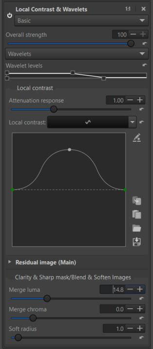
• In Selective Editing, there is the Local Contrast & Wavelets tool, which in Basic mode allows you to adjust the local contrast (by choosing the appropriate range of decomposition levels) along with a Clarity function.